
Linear Regression Using Gradient Decent
When it comes to machine learning a popular starting place tends to be linear regression using gradient descent. The reasoning is that it is a simple optimization problem, that is easy to understand and helps to gradually introduce a common topic in machine learning.
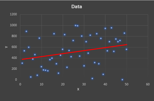
Many of you are probably familiar with linear regression; the process of making a line correlating scattered data (see figure below). Linear regression is useful to so many applications. Whether you are trying to predict the inflationary price increases at the supermarket, or you are trying to predict how high a person can jump based on their height, the usefulness of linear regression spans seemingly endless domains.
As a gradual introduction to machine learning, we will discuss how to perform a linear regression (line fitting approximation) on a set of 2-D data (X & Y) utilizing a gradient descent algorithm.
For us to make use of this technique, we must understand two fundamental things. First, what is linear regression? Second, what is gradient descent? Most of you are probably familiar with the prior, so I will speed through that portion and focus on the lesser-known gradient descent portion.
First, we discuss linear regression. Simply put, linear regression is a line-fitting technique to fit a line onto scattered data. The goal is to create a line-based model that can be used to predict a value based on one or more other values.
Linear regression (in the 2-D case) involves the classic equation for a line as shown below.
y=m * x + b
Where m represents the slope of the line, and b represents the y-intercept.
The goal of linear regression is to find values for m & b that allow the line to best fit (model) the scattered data (if the scattered data were to be a line). The figure above provides an illustration of an approximate line fit (linear regression) for the scattered data in the plot.
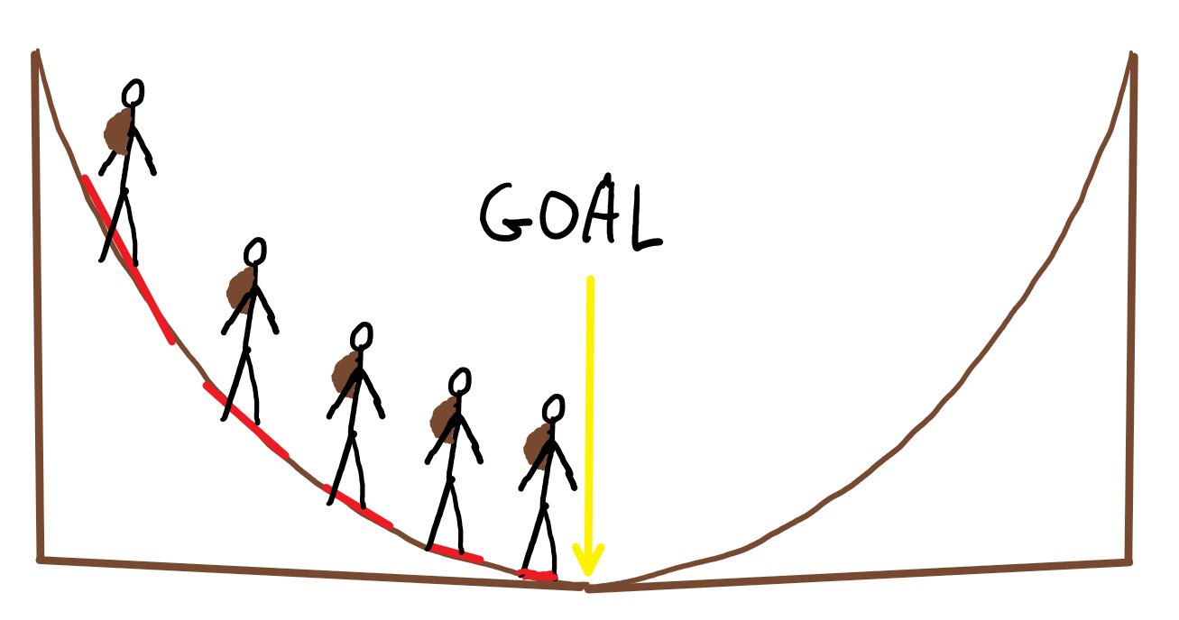
Second, we discuss gradient descent. Gradient descent is a recursive optimization algorithm that is utilized to find the minimum of a function. To illustrate this conceptually, let's imagine a hiker walking down the slope of a hill, to reach the bottom. When the hiker starts, he will take large steps, however, as he approaches his goal, he will begin to take smaller and smaller steps to prevent passing his goal.
Example of a line produced by linear regression.
In the case of the hiker, the value he is trying to minimize is the distance between himself and the bottom of the hill. In the case of linear regression, the value we are trying to minimize is the error between each of the y-values in the scatter plot. This can be expressed in terms of an equation called a Loss Function.
E = 1/n * summation[i=0][n-1]{(yi - mean(yi))^2}
Since we know the mean will our line equations, we can derive the following.
E = 1/n * summation[i=0][n-1]{(yi - (m * xi + b))^2}
Now that we know what we are minimizing, we can introduce our iterative approach to doing so. Since our error function has two independent variables (m and b) we need to adjust the values to minimize our error. To adjust these values with our gradient descent algorithm, we need to use the following formulas.
m = m - Lm
b = b - Lb
In these formulas, L is an arbitrary learning rate constant and is the result of the partial derivatives of our loss function. The learning rate can be thought of as a negative gain factor that controls the convergence speed and accuracy of the algorithm. As you probably guessed, we are going to derive the formulas for the partial derivates of our loss function concerning these two independent variables. The partial derivatives are shown below.
Dm = -2/n * summation[i=0][n-1](yi - (m * xi + b))(xi)
Db = -2/n * summation[i=0][n-1](yi - (m * xi + b))
Now that we have derived all of our equations we can utilize them to perform a gradient decent linear regression with the following steps:
Initially set m and b to be 0, and set our learning rate to a constant 0.0001. Having a small learning rate like this will allow for greater accuracy. Since our algorithm is small, this will have minimal impact on the speed with which our implemented program will converge.
Next, we calculate the partial derivate values.
Next, we calculate our new m and b values.
Finally, we calculate the loss function error. We will terminate our algorithm when our loss function reaches an error of zero or some very small value. Upon termination, the values of m and b will provide us with our linear regression line equation.